Variant surveillance example
Source:vignettes/V6_IllustrativeExample.Rmd
V6_IllustrativeExample.RmdIn this vignette, we use the phylosamp package to
prepare for the emergence of a new variant of a SARS-CoV-2-like pathogen
into a fictional population, based on current whole genome sequencing
capacity and experience with previous variants of concern.
There are three steps in applying our method:
Determine the population of interest (Figure 1). In this example, we’ll assume we are interested in tracking variants of Pathogen X in a small country with a well-defined population.
Identify the key question we are trying to answer with our surveillance scheme. In this example, we will assume we are interested in calculating the sample size needed to detect the emergence of a new variant of Pathogen X by the time it reaches a frequency of 1% across all infected individuals in our country. In other words, we will focus on variant detection.
Identify the sampling frequency we have the capacity to maintain. In our case, we’ll assume we want to develop a weekly sampling scheme, in which pathogen samples collected over a 7-day period are sequenced in weekly batches (i.e., periodic surveillance).
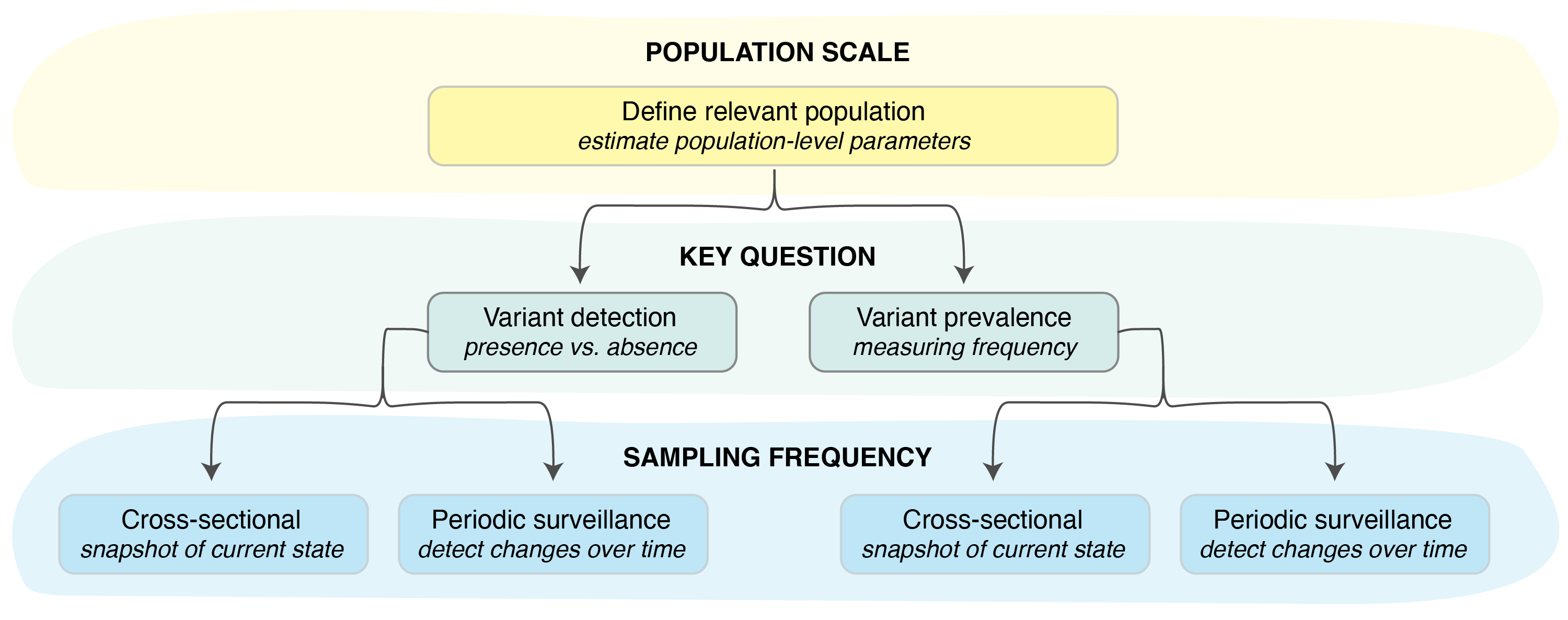
Figure 1. Key steps in setting up a pathogen surveillance system.
Now that we’ve identified our surveillance goals, we need to estimate some basic parameters for our population of interest, such as the pathogen testing rate, the sensitivity of the tests used, etc. However, since these values may vary by pathogen variant, we need to explore and estimate these parameters in a variant-specific context. In the current implementation of the sample size calculation methodology described herein, the specific parameters we will need to consider are (see Table 1): the variant-specific asymptomatic rate, the asymptomatic and symptomatic testing rates, the variant-specific testing sensitivity using currently available technologies, the variant-specific sampling success rate (i.e., the expected number of samples of high enough quality for variant characterization by whole genome sequencing), and the sequencing success rate. Let’s consider each of these parameters in turn (see also: Estimating bias in observed variant prevalence).
Guidance for determining variant-specific parameters
The asymptomatic rate (\(\psi\)).
- So far, epidemiologists have determined that the asymptomatic rate of Pathogen X has ranged from 30-40%. The currently circulating variant has an asymptomatic rate of 30%. Given this, we want to plan for variants that could have asymptomatic rates ranging from 25-45%. A lower asymptomatic rate causes enrichment of the variant in sampled infections; conversely, a higher asymptomatic rate would artificially deplete samples belonging to the variant of interest in the pool of detected infections. Therefore, an asymptomatic rate of 25% represents the least conservative scenario (since enrichment of a variant of interest would mean fewer sequences are required to detect it) while an asymptomatic rate of 45% represents the most conservative scenario.
The testing rate (\(\tau\)).
- Given the widespread availability of rapid antigen tests for Pathogen X, we assume that only 50% of symptomatic infections (of any variant) are tested, and only 10% of asymptomatic infections are detected and samples sent to national public health laboratories. We anticipate that testing rates could drop as low as 40% (symptomatic) / 5% (asymptomatic) as the population becomes increasingly desensitized to disease spread. Because of the complex relationship between testing rates and sampling bias, we’ll explore these two scenarios independently when performing sample size calculations.
The testing sensitivity (\(\phi\)).
- The current gold-standard PCR test for Pathogen X has a sensitivity of 95% for the currently circulating variant. Historical data shows this rate has changed very little between variants. However, to account for the possibility that a future variant may significantly change the viral load present in patient samples or mutate in such a way that tests temporarily become less effective (until an updated PCR target can be developed), we will perform sample size calculations assuming no change in sensitivity (least conservative scenario) as well as a drop in sensitivity down to 90% (most conservative scenario).
The sampling success rate (\(\gamma\)).
- In many laboratory settings, viral load is measured for each sample by qPCR prior to sequencing, and the results are used to select samples for sequencing. Only sequencing the highest quality samples ensures the sequencing process is maximally cost effective. For the sake of example, we will assume that the sampling success rate is expected to be the same across all potential variants. However, we can imagine that a variant with a lower sampling success rate would require additional sampling for accurate detection.
The sequencing success rate (\(\omega\)).
- Not all samples selected for sequencing will produce high quality genomes that can be used for variant characterization. We assume that sequencing success is fixed across all variants, as the factors that affect sequencing success are not independent of those affecting infection detection and sample quality. In the national laboratory of our country of interest, the sequencing success rate is 80%.
The coefficient of detection ratio
Once we have estimated the parameter ranges of interest, we can
calculate the coefficient of detection in the most and
least conservative scenarios. We can do this using the
vartrack_cod_ratio() function as shown below (for more
details, see Estimating
bias in observed variant prevalence).
When calculating the coefficient of detection, keep in mind that the \(\gamma\) parameter can be left out for both the variant of interest and general population parameters, since (as discussed above) we are assuming that this parameter does not change between variants. In the least conservative scenario as described above, the testing sensitivity \(\phi\) also does not differ between potential new variants and the currently circulating pathogen population.
We can provide the remaining parameters as follows. (Note that \(V_1\) represents the future variant we want to capture and \(V_2\) parameters correspond to the general pathogen population.)
library(phylosamp)

# Least conservative scenario assuming higher testing rate:
vartrack_cod_ratio(psi_v1=0.25, psi_v2=0.3, tau_a=0.1, tau_s=0.5)
## [1] 1.052632
# Least conservative scenario assuming lower testing rate:
vartrack_cod_ratio(psi_v1=0.25, psi_v2=0.3, tau_a=0.05, tau_s=0.4)
## [1] 1.059322
# Most conservative scenario assuming higher testing rate:
vartrack_cod_ratio(psi_v1=0.45, psi_v2=0.3, phi_v1=0.9, phi_v2=0.95,
                   tau_a=0.1, tau_s=0.5)
## [1] 0.7977839
# Most conservative scenario assuming lower testing rate:
vartrack_cod_ratio(psi_v1=0.45, psi_v2=0.3, phi_v1=0.9, phi_v2=0.95,
                   tau_a=0.05, tau_s=0.4)
## [1] 0.778769Given these results, we can move forward to sample size calculations with two values of the coefficient of detection ratio to test: 0.779 (most conservative scenario) and 1.059 (least conservative scenario).
Sample size calculations
Once we have determined the range of scenarios we’d like to explore,
we can perform sample size calculations. As our aim is to ensure variant
detection using a periodic sampling strategy, we need to use the
sampling_freq = "cont" option of the
vartrack_samplesize_detect() function of the
phylosamp R package (see Estimating the sample size
needed for variant monitoring: periodic sampling for
more details).
To do this, there are a few more parameters we need to estimate:
The desired probability of detection (\(prob\)).
- We can again select a parameter range to explore for our sample size calculations. In our case, we want to ensure a good chance of detecting a new variant of Pathogen X when it enters our country, so we will explore probabilities of detection between 75% (least conservative) to 95% (most conservative).
The desired variant prevalence (\(p_{\text{detect}}\)).
- As stated above, we want to ensure we catch any variant by the time it has reached 1% prevalence in the population of infected individuals.
Initial variant prevalence (\(p_0\)).
- The method we will use for sample size calculations assumes logistic growth of any new variants of concern, with a starting prevalence and growth rate that can be specified. This initial prevalence depends on the number of simultaneous variant introductions into our country of interest as well as the total infected population size. Over the last year, we have observed a total of between 5,000 and 10,000 total cases of Pathogen X in our country at any given time, and we expect the number of cases to be similar if a new variant is introduced. Because of the complex relationship between initial prevalence and the shape of the logistic growth curve, we will estimate the required sample size in two scenarios: (1) if a new variant could be introduced via a single index case, at a time when nearly 10,000 people are infected (initial prevalence \(=1/10000\)); and (2) if 5 different travelers are be infected by a new variant and bring it into the country in the same week, at a time when only 5,000 individuals are infected (initial prevalence \(=5/5000=1/1000\)).
Logistic growth rate (\(r\)).
- We also need to estimate a variant growth rate over time. Based on historical data of Pathogen X, we know that a recently introduced variant may grow as slowly as 0.1x/day (least conservative, as fewer samples are needed to ensure we catch the variant before it goes above 1% frequency) or as quickly as 0.2x/day (most conservative).
We now have all of the values we need to estimate the sample size
needed for detecting a variant by the time it reaches 1% in the
population, assuming weekly periodic sampling. Additionally, it is
important to remember that the number of required
sequences is not the same as the number of required
samples, because of the sequencing success rate (\(\omega\)) discussed above. The
phylosamp functions output the number of samples required,
taking into account that not all samples selected for sequencing will
result in high quality samples suitable for variant
characterization:
library(phylosamp)

# Least conservative scenario with low initial prevalence:
vartrack_samplesize_detect(prob=0.75, p_v1=0.01, p0_v1=1/10000, r_v1=0.1,
                           omega=0.8, c_ratio=1.059, sampling_freq="cont")
## Calculating sample size for variant detection assuming periodic sampling## [1] 15.106
# Least conservative scenario with high initial prevalence:
vartrack_samplesize_detect(prob=0.75, p_v1=0.01, p0_v1=1/1000, r_v1=0.1,
                           omega=0.8, c_ratio=1.059, sampling_freq="cont")
## Calculating sample size for variant detection assuming periodic sampling## [1] 16.41287
# Most conservative scenario with low initial prevalence:
vartrack_samplesize_detect(prob=0.95, p_v1=0.01, p0_v1=1/10000, r_v1=0.2,
                           omega=0.8, c_ratio=0.779, sampling_freq="cont")
## Calculating sample size for variant detection assuming periodic sampling## [1] 80.14972
# Most conservative scenario with high initial prevalence:
vartrack_samplesize_detect(prob=0.95, p_v1=0.01, p0_v1=1/1000, r_v1=0.2,
                           omega=0.8, c_ratio=0.779, sampling_freq="cont")
## Calculating sample size for variant detection assuming periodic sampling## [1] 96.2708Based on these calculations, we need to be sequencing between 16 and 97 samples per day (or 112 and 679 samples per week) in order to detect a new variant by the time it reaches 1% in the population. As this is a rather wide range, we can use the reverse functionality of the sample size calculation method to determine the probability of detecting a variant given a fixed number of samples and most conservative parameter values.
Estimating the probability of detection
Given the recommendation of 112-679 samples per week, the government
of our country of interest has decided that funding will be allocated to
support sequencing of 200 Pathogen X samples per week. Given our most
conservative scenario of a coefficient of detection of 0.779 and a
growth rate of 0.2, we can use the vartrack_prob_detect()
function to calculate the probability of detecting a variant before it
crosses the 1% prevalence threshold in the population (see
Estimating the probability of detecting a variant: periodic sampling).
library(phylosamp)

# Most conservative scenario with low initial prevalence
vartrack_prob_detect(n=28, p_v1=0.01, p0_v1=1/10000, r_v1=0.2,
                     omega=0.8, c_ratio=0.779, sampling_freq="cont")
## Calculating probability of detection assuming periodic sampling## [1] 0.6488521
# Most conservative scenario with high initial prevalence
vartrack_prob_detect(n=28, p_v1=0.01, p0_v1=1/1000, r_v1=0.2,
                     omega=0.8, c_ratio=0.779, sampling_freq="cont")
## Calculating probability of detection assuming periodic sampling## [1] 0.5815917In both the high and low initial prevalence scenarios, the probability of detection (assuming roughly 28 samples selected per day, to be sequenced in weekly batches) remains above 58% even using the most conservative parameters. Furthermore, the probability of detecting a new variant by the time it reaches 2% in the population is approximately 85% in both scenarios (as shown below), with numbers approaching 99% chance of detection before the variant hits 5% prevalence. These values may be sufficient for country officials to feel confident in their ability to detect a variant soon after it is introduced regardless of its biological properties; if it is not, the calculations can simply be repeated with a higher number of weekly samples.
library(phylosamp)

## DETECTION BEFORE REACHING 2% PREVALENCE

# Most conservative scenario with low initial prevalence
vartrack_prob_detect(n=28, p_v1=0.02, p0_v1=1/10000, r_v1=0.2,
                     omega=0.8, c_ratio=0.779, sampling_freq="cont")
## Calculating probability of detection assuming periodic sampling## [1] 0.8514334
# Most conservative scenario with high initial prevalence
vartrack_prob_detect(n=28, p_v1=0.02, p0_v1=1/1000, r_v1=0.2,
                     omega=0.8, c_ratio=0.779, sampling_freq="cont")
## Calculating probability of detection assuming periodic sampling## [1] 0.8693221
## DETECTION BEFORE REACHING 5% PREVALENCE

# Most conservative scenario with low initial prevalence
vartrack_prob_detect(n=28, p_v1=0.05, p0_v1=1/10000, r_v1=0.2,
                     omega=0.8, c_ratio=0.779, sampling_freq="cont")
## Calculating probability of detection assuming periodic sampling## [1] 0.9940441
# Most conservative scenario with high initial prevalence
vartrack_prob_detect(n=28, p_v1=0.05, p0_v1=1/1000, r_v1=0.2,
                     omega=0.8, c_ratio=0.779, sampling_freq="cont")
## Calculating probability of detection assuming periodic sampling## [1] 0.989769Of course, there are many assumptions that underlie these calculations, the most obvious being that the weekly batch of samples for sequencing are assumed to be well-distributed across the days of the week, and that they capture all regions or ports of entry into the country. Even so, this method provides sampling guideposts that can be applied in a variety of settings. For example, it is clear from the simple calculations above that 100 samples per week would be unlikely to be particularly informative for detecting new variants early and with high confidence.
Although the example provided here focuses on the question of detection with periodic sampling, the same principles (though different functions/spreadsheet tabs) can be applied to a cross-sectional sampling scheme (see Estimating the sample size needed for variant monitoring: cross-sectional and Estimating the probability of detecting a variant: cross-sectional) and/or estimating variant prevalence. The section on the coefficient of detection remains identical, and only the sampling calculations need to be updated to suit the surveillance goals.