Estimating the probability of detecting a variant

Cross-sectional sampling

In this vignette we discuss how the variant tracking functions can be used in reverse, to calculate the probability or confidence of detection (or effective prevalence estimation) given a fixed sample size. In other words, if we have a predetermined number of infections we can sequence or otherwise characterize, we can use the phylosamp package to determine the probability we will detect or correctly estimate the prevalence of a known pathogen variant.

Variant detection

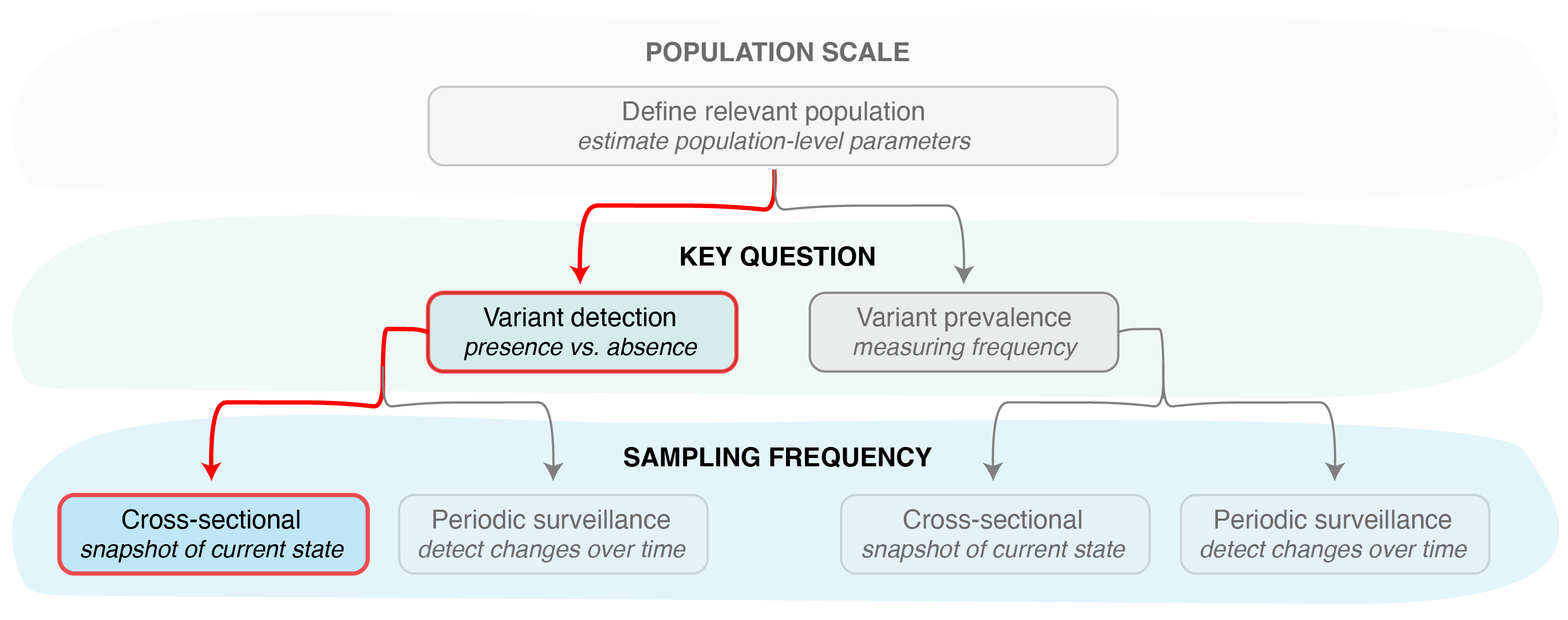
Figure 1. Identifying the key question (detection vs prevalence) is the second step in designing a pathogen surveillance system. Determining confidence in the result (e.g., the probability of detection or confidence in frequency estimation) then requires determining the sampling frequency (cross-sectional or periodic).

We can use the vartrack_prob_detect() function with the sampling_freq = "xsect" option for calculating the probability of detecting a circulating variant at a specific prevalence level, given a cross-sectional sample of fixed size (Figure 1). Like it’s inverse function (vartrack_samplesize_detect(); see Estimating the sample size needed for variant monitoring: cross-sectional sampling), this function requires knowledge of the coefficient of detection ratio between two pathogen variants (or, more commonly, one variant and the rest of the pathogen population). The coefficient of detection ratio for two variants can be calculated using the vartrack_cod_ratio() function (see Estimating bias in observed variant prevalence for more details). Since we are only interested in the ratio of the coefficients of detection, applying this function only requires providing parameters which are expected to differ between variants. The ratio between any variants not provided is assumed to be equal to one.

Once we have an estimate of the coefficient of detection ratio, we can calculate the probability of detection from the following parameters:

Param	Variable Name	Description
\(P_{V_1}\)	p_v1	the desired minimum variant prevalence to be able to detect
\(n\)	n	the sample size
\(\omega\)	omega	the sequencing success rate
\(\frac{C_{V_1}}{C_{V_2}}\)	c_ratio	the coefficient of detection ratio, calculated as the ratio of the coefficients of variant 1 to variant 2 (can be calculated using vartrack_cod_ratio())

We then apply this probability calculation function as follows:

library(phylosamp)

c1_c2 <- vartrack_cod_ratio(phi_v1=0.975, phi_v2=0.95, gamma_v1=0.8, gamma_v2=0.6)
vartrack_prob_detect(p_v1=0.02, n=100, omega=0.8, c_ratio=c1_c2, sampling_freq="xsect")

## Calculating probability of detection assuming single cross-sectional sample

## [1] 0.8895872

In other words, we have an 89% probability of detecting a variant at 2% (or higher) in a population given a sample size of 100 samples selected for sequencing. In this calculation, we assumed that only 80% (\(\omega=0.8\)) of samples sequenced (or otherwise characterized) are successful, leading to an effective sample size of 80 samples. We also calculated a coefficient of detection ratio (\(\frac{C_{V_1}}{C_{V_2}}\)) of 1.368, which increased our confidence in detecting the variant, since we expect it to be enriched in the population of detected infections.

Once again, this probability of detection assumes samples are collected roughly all at once, providing a cross-sectional picture of the circulating variant(s). For information on functions that can be used to determine the probability of detection given a periodic sampling approach, see Estimating the sample size needed for variant monitoring: periodic sampling. To estimate the sample size given some desired probability of detection see the Estimating the sample size needed for variant monitoring cross-sectional and periodic vignettes.

Variant prevalence

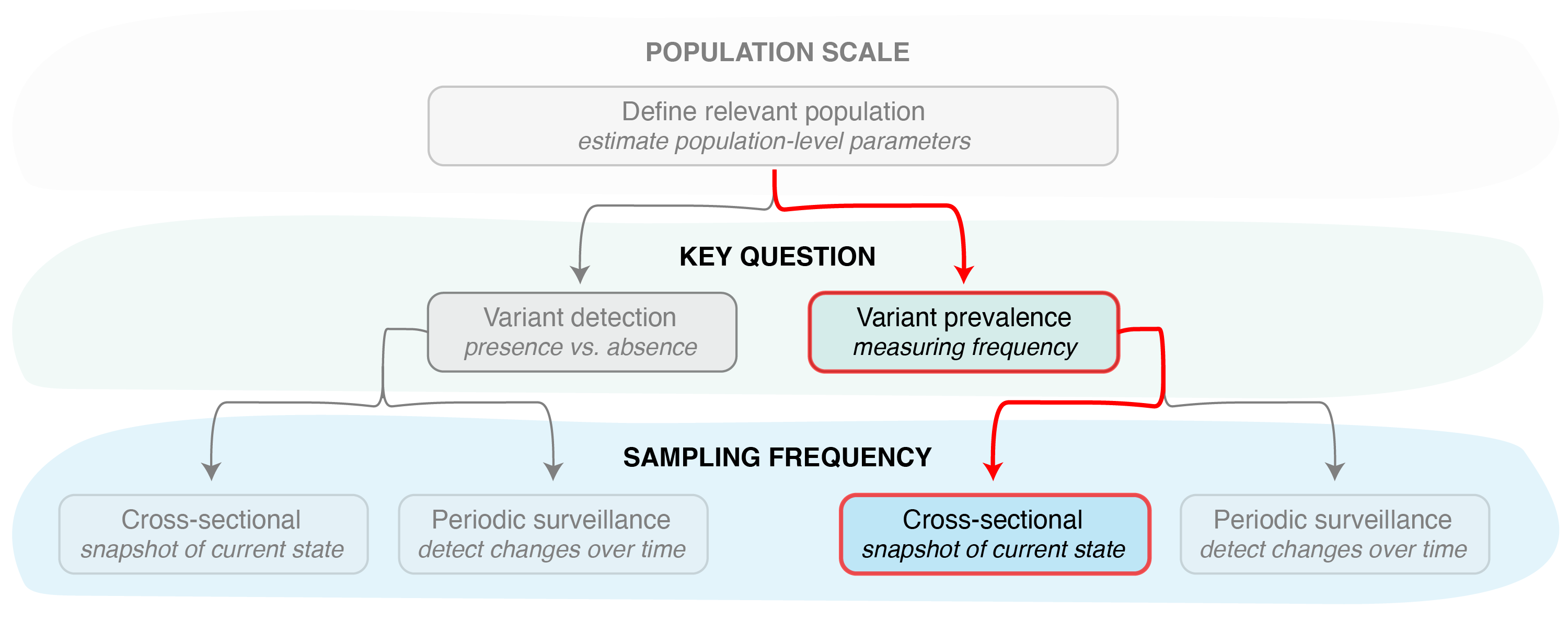
Figure 2. Other functions in the phylosamp package can be used to determine the confidence in our variant prevalence estimate, again assuming a single cross-sectional sample.

In some cases, we may be more interested in correctly estimating the variant frequency than simply stating its presence or absence in the population (Figure 2). In this case, we can use the vartrack_prob_prev() function to determine our confidence in our estimate of variant prevalence given a fixed sample size. This function requires the user to specific a slightly different set of parameters:

Param	Variable Name	Description
\(P_{V_1}\)	p_v1	the desired minimum variant prevalence
\(n\)	n	the sample size
\(\omega\)	omega	the sequencing success rate
\(d\)	precision	the desired precision in the prevalence estimate
\(\frac{C_{V_1}}{C_{V_2}}\)	c_ratio	the coefficient of detection ratio, calculated as the ratio of the coefficients of variant 1 to variant 2 (can be calculated using vartrack_cod_ratio())

We then can calculate confidence in the estimated prevalence as follows:

c1_c2 <- vartrack_cod_ratio(psi_v1=0.25, psi_v2=0.4, tau_a=0.05, tau_s=0.3)
vartrack_prob_prev(p_v1=0.1, n=200, omega=0.8, precision=0.25, 
                   c_ratio=c1_c2, sampling_freq="xsect")

## Calculating confidence in variant estimate assuming single cross-sectional sample

## [1] 0.7493082

In other words, we can be 75% confident that any estimate of prevalence of a variant we expect has at least 10% prevalence in the population is within 25% of the true value, given a sample size of 200 samples. This takes into account the fact that we expect only 80% (\(\omega=0.8\)) of these samples will be successfully sequenced (or otherwise characterized). It also assumes that our variant of interest has a lower asymptomatic rate than the rest of the pathogen population (\(\psi_{V_1}=0.25\) vs \(\psi_{V_2}=0.4\)) and that the testing probability of symptomatic infections (\(\tau_s=0.3\)) is 6 times higher than the testing probability of asymptomatic infections (\(\tau_a=0.05\)), leading to a coefficient of detection ratio of 1.188.

Other sampling scenarios

Currently, the phylosamp package does not provide functionality for estimating the probability of accurately estimating variant prevalence given a periodic sampling approach (though this functionality is implemented for the probability of detection, see Estimating the sample size needed for variant monitoring: periodic sampling).

The package contains functionality for determining the required sample size for both detection and prevalence estimation, in the Estimating the sample size needed for variant monitoring cross-sectional and periodic vignettes.