Estimating the sample size needed for variant monitoring

Periodic sampling

This vignette provides an overview of the functions that can be used to estimate the sample size needed to detect a pathogen variant in a population, given a periodic sampling scheme.

Variant detection

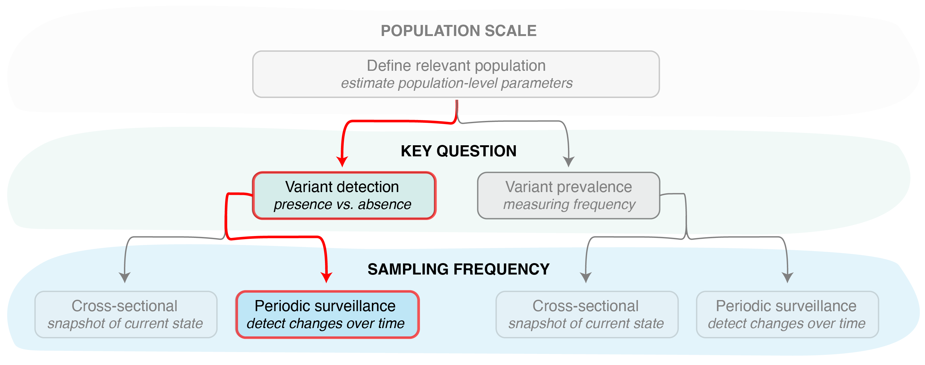
Figure 1. Identifying the key question (detection vs prevalence) is the second step in designing a pathogen surveillance system. Determining the sample size needed to answer this question then requires determining the sampling frequency, i.e., if samples will be collected and sequenced just once (cross-sectional sampling) or with some regularity over a period of time (periodic surveillance).

By specifying sampling_freq = "cont", the vartrack_samplesize_detect() function can be used to calculate the sample size needed to detect a particular variant in the population within a specific number of days since its introduction, OR by the time a variant reaches a specific frequency. As when specifying cross-sectional sampling with sampling_freq = "xsect" (see Estimating the sample size needed for variant monitoring: cross-sectional sampling for details), applying the vartrack_samplesize_detect() function to calculate a sample size assuming periodic sampling (Figure 1) requires knowledge of the coefficient of detection ratio between two pathogen variants (or, more commonly, one variant and the rest of the pathogen population). The coefficient of detection ratio for two variants can be calculated using the vartrack_cod_ratio() function (see Estimating bias in observed variant prevalence). Since we are only interested in the ratio of the coefficients of detection, applying this function only requires providing parameters which are expected to differ between variants. The ratio between any variants not provided is assumed to be equal to one.

Once we have an estimate of the coefficient of detection ratio, we can calculate the sample size needed for detection from the following parameters:

Param	Variable Name	Description
\(p\)	prob	the desired probability of detection
\(t\)	t	the number of days after introduction a variant should be detected by
\(P_{V_1}\)	p_v1	the desired prevalence to detect a variant by
\(P_{0_{V_1}}\)	p0_v1	the initial variant prevalence (# introductions / population size)
\(r_{V_1}\)	r_v1	the estimated logistic growth rate of the variant (per day)
\(\omega\)	omega	the sequencing success rate
\(\frac{C_{V_1}}{C_{V_2}}\)	c_ratio	the coefficient of detection ratio, calculated as the ratio of the coefficients of variant 1 to variant 2 (can be calculated using calc_cod_ratio())

To calculate the sample size needed for detection assuming periodic sampling, we must provide either the number of days after introduction a variant should be detected by (\(t\)) OR the desired prevalence to detect a variant by (\(P_{V_1}\)), but not both. All other parameters listed above are required.

Therefore, if we would like to know the sample size needed per day to ensure detection of a variant by the time it reaches 1% prevalence in the population, we can apply the vartrack_samplesize_detect() function as follows:

library(phylosamp)

c1_c2 <- vartrack_cod_ratio(phi_v1=0.975, phi_v2=0.95, gamma_v1=0.8, gamma_v2=0.6)
vartrack_samplesize_detect(prob=0.95, p_v1=0.01, p0_v1=3/10000, r_v1=0.1, 
                           omega=0.8, c_ratio=c1_c2, sampling_freq="cont")

## Calculating sample size for variant detection assuming periodic sampling

## [1] 25.81341

In other words, 26 samples per day are needed to detect a variant at 1% (or higher) in a population with 95% probability of detection, given a coefficient of detection ratio (\(\frac{C_{V_1}}{C_{V_2}}\)) of 1.368 (as calculated from parameters listed above). This assumes that all samples sequenced (or otherwise characterized) will be successful. We assume an 80% success rate (\(\omega = 0.8\)), which ensures the 21 high quality data points that can be used to detect the presence of a pathogen variant from a selection of 27 samples. If sequencing will occur on a weekly basis, this means we need to process \(26*7=182\) samples per week (ideally from infections spread evenly over the 7 days) to ensure we detect a variant by the time it reaches 1% frequency in the population.

Variant prevalence

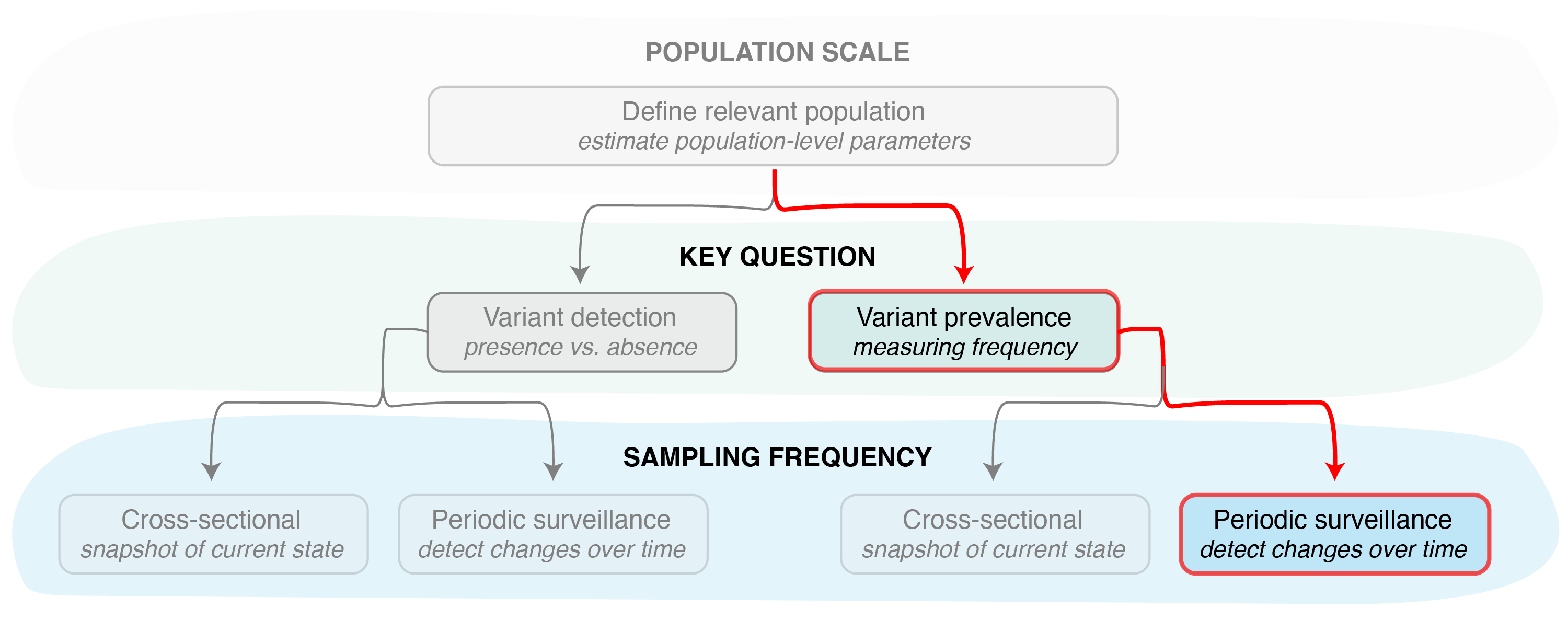
Figure 2. Other functions in the phylosamp package can be used to determine the sample size needed to accurately monitor variant prevalence given a periodic sampling strategy.

If instead we are interested in detecting a variant within the first month of its introduction into the population (assuming all other parameters are the same as above), we can use the vartrack_samplesize_detect() function as follows:

c1_c2 <- vartrack_cod_ratio(phi_v1=0.975, phi_v2=0.95, gamma_v1=0.8, gamma_v2=0.6)
vartrack_samplesize_detect(prob=0.95, t=30, p0_v1=3/10000, r_v1=0.1, 
                           omega=0.8, c_ratio=c1_c2, sampling_freq="cont")

## Calculating sample size for variant detection assuming periodic sampling

## [1] 47.98564

In this case, we can see that we will need to process 48 samples per day (which, assuming an 80% sequencing success rate, means generating 39 high quality sequences per day) to ensure detection within the first month of variant introduction into the population.

Other sampling scenarios

For information on functions that can be used to estimate the sample size given a cross-sectional sampling approach, see Estimating the sample size needed for variant monitoring: cross-sectional sampling. These functions can also be used in “reverse”, to calculate the probability of detection given some sampling scheme, as in the Estimating the probability of detecting a variant cross-sectional and periodic vignettes.