Illustrative examples for evaluating transmission linkage • phylosamp

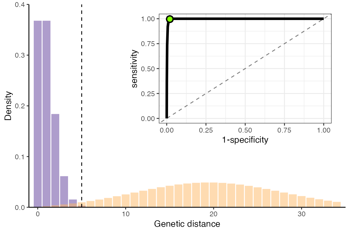
In this vignette, we apply the functions provided to estimate sensitivity and specificity and apply them to an Ebola-like pathogen. We compare the results to those of a pathogen with a slower mutation rate and higher reproductive number. Then, we will use these results to calculate the false discovery rate of our linkage criteria (genetic distance) given a sample size of 200 and a relevant population of 1000 infected individuals.

In the first part of this vignette, we use the function gendist_roc_format(), which formats the results of gendist_sensspec_cutoff() for plotting ROC curves.

library(phylosamp)
library(ggplot2)
library(RColorBrewer)
library(cowplot)

Calculating sensitivity and specificity for an Ebola-like pathogen

# ebola-like pathogen
R <- 1.5
mut_rate <- 1

# use simulated generation distributions
data("genDistSim")
mean_gens_pdf <- as.numeric(genDistSim[genDistSim$R == R, -(1:2)])

# get theoretical genetic distance dist based on mutation rate and generation parameters
dists <- as.data.frame(gendist_distribution(mut_rate = mut_rate, 
                                            mean_gens_pdf = mean_gens_pdf, 
                                            max_link_gens = 1))

# reshape dataframe for plotting
dists <- reshape2::melt(dists, 
                        id.vars = "dist", 
                        variable.name = "status", 
                        value.name = "prob")

# get sensitivity and specificity using the same paramters
roc_calc <- gendist_roc_format(cutoff = 1:(max(dists$dist)-1), 
                               mut_rate = mut_rate,
                               mean_gens_pdf = mean_gens_pdf)
  
# get the optimal value for the ROC plot
roc_optim <- optim_roc_threshold(roc_calc)
threshold <- roc_optim$cutoff
optim_point <- c(roc_optim$specificity, roc_optim$sensitivity)

# plot the distributions of genetic distance
pal <- RColorBrewer::brewer.pal(5, "PuOr")
  
p1 <- ggplot(dists, aes(x=dist, y=prob, fill=status)) +
    geom_bar(alpha=0.5, stat="identity", position="identity") +
    scale_fill_manual(name="", values=c(pal[5], pal[2])) +
    scale_x_continuous(limits = c(-1,35), expand = c(0,0)) +
    scale_y_continuous(limits = c(0,0.4), expand = c(0,0)) +
    xlab('Genetic distance') + ylab('Density') +
    theme_classic() + theme(legend.position='none') +
    geom_vline(xintercept=threshold, linetype=2, size=0.5, color = "black")
  
# add ROC curve on top
r1 <- ggplot(data=roc_calc, aes(x=specificity, y=sensitivity)) +
    geom_line(size=1.5) + xlim(0,1) + ylim(0,1) +
    geom_point(x=optim_point[1], y=optim_point[2],
               size = 3, stroke=1, shape=21, fill = "chartreuse") +
    geom_abline(slope=1, intercept = 0, linetype=2, alpha=0.5) +
    xlab("1-specificity") +
    theme_bw()
  
cowplot::ggdraw(p1) + cowplot::draw_plot(r1, hjust=-0.16, vjust=-0.16, scale=0.6)

Optimal values for an Ebola-like pathogen

Using the closest-to-corner method, the optimal genetic distance threshold for this pathogen is:

threshold

## [1] 5

And the sensitivity and specificity at this threshold is:

roc_optim$sensitivity ## sensitivity

## [1] 0.9963402

1 - roc_optim$specificity ## specificity

## [1] 0.9801562

Calculating sensitivity and specificity for a faster-spreading, slower mutating pathogen

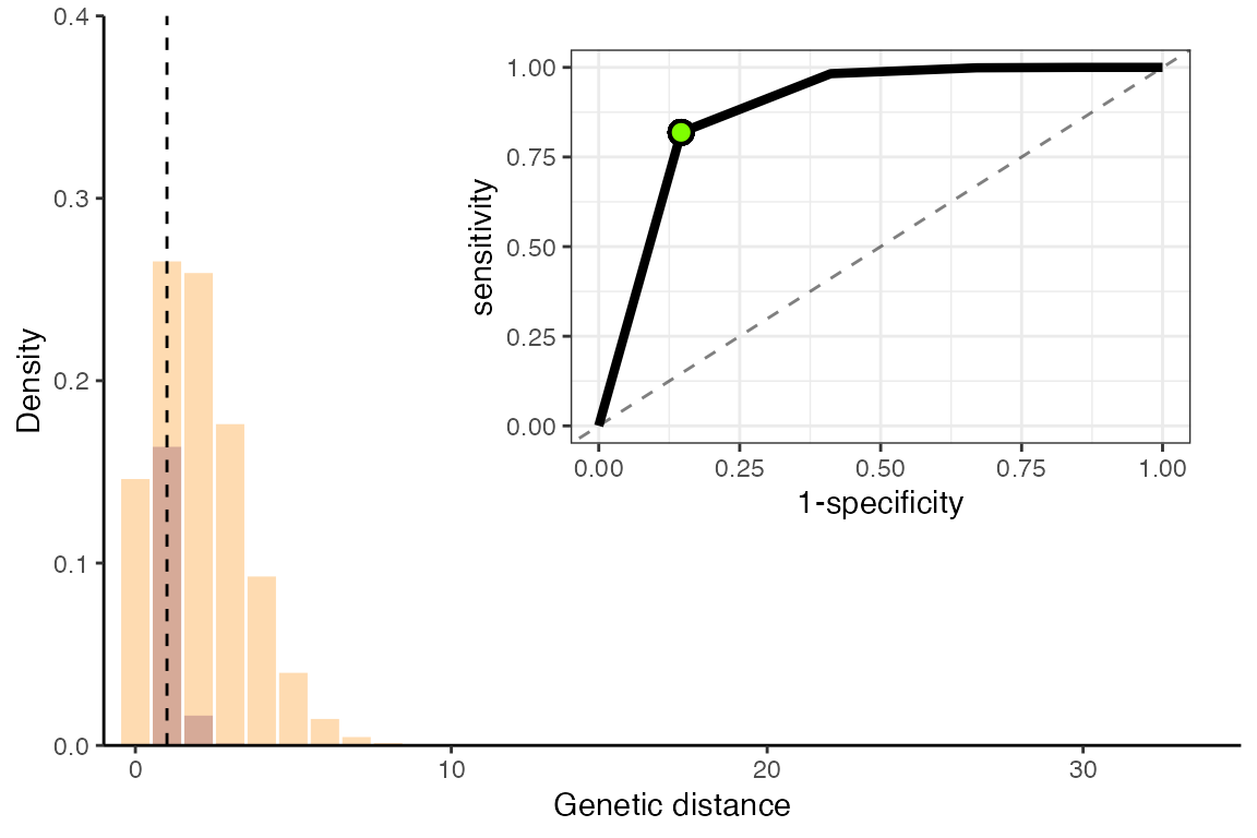
We repeat the above plot for a pathogen with a higher reproductive number and lower mutation rate:

# faster-spreading pathogen
R <- 3
mut_rate <- 0.2

mean_gens_pdf <- genDistSim[genDistSim["R"]==R][3:dim(genDistSim)[2]]

Optimal values for a faster-spreading, slower mutating pathogen

For this pathogen, the optimal genetic distance threshold is:

threshold

## [1] 1

And the sensitivity and specificity at this threshold is:

roc_optim[roc_optim$cutoff==threshold,]$sensitivity ## sensitivity

## [1] 0.8187308

1 - roc_optim[roc_optim$cutoff==threshold,]$specificity ## specificity

## [1] 0.8539157

It is well understood that genetic distance is a much more accurate predictor of transmission linkage for pathogens with higher mutation rates and slower spread, as shown clearly in this example (lower sensitivity and specificity in the second example). Genetic distance is clearly not an appropriate metric for all pathogens, but more sophisticated linkage criteria – especially those that incorporate epidemiological information as well – may produce better results.

Calculating the false discovery rate of genetic distance as a linkage criteria

This is reflected in our confidence in identifying linked infection pairs. Assuming a sample size of 200, a relevant population of 1000, and the genetic distance threshold and associated sensitivity and specificity for each pathogen we get:

translink_tdr(sensitivity=0.9963402, specificity=0.9801562, 
              rho=0.20, M=200, R=1) # ebola-like pathogen

## Calculating true discovery rate assuming multiple-transmission and multiple-linkage

## [1] 0.09183886

translink_tdr(sensitivity=0.8187308, specificity=0.8539157, 
              rho=0.20, M=200, R=1) # slower-mutating pathogen

## Calculating true discovery rate assuming multiple-transmission and multiple-linkage

## [1] 0.01116204

As a final note, we remind the reader that the specificity of the linkage criteria has a significant bearing on the true/false discovery rate, and that high true discovery rates require a specificity upwards of 0.999. Linkage criteria more complex than genetic distance may be needed to achieve this value.